6. Classification using ENVI 5.5

6.1. Aims

After completing this practical, you should be able to analyse one or more image datasets using classification methods. This includes learning to identify land cover classes in a dataset and consider class separability (using histograms, scatterplots and other tools), and applying and assessing a classification product using Envi.

6.2. Introduction

The datasets you need for this practical are available from the `Classification data (Rondônia) folder on moodle <>`__ or you can download them individually:

https://moodle.ucl.ac.uk/mod/folder/view.php?id=2749790 * ETM-110801 * ETM-110801.HDR * TM-250792 * TM-250792.HDR

With accompanying elevation data * SRTM-2002 * SRTM-2002.HDR

You should download these data and put them in a directory (folder) that you will remember!

See Classification Introduction for more details on the context and datasets.

6.3. Examination of the data

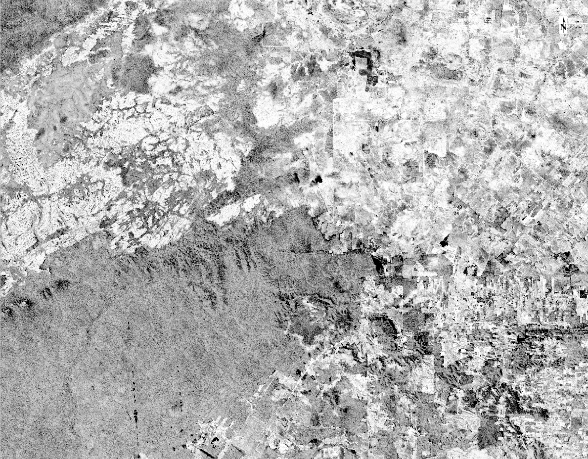
Load up the two images and examine the data. Try to identify the various classes you might like to obtain for this exercise decide how you can identify them. Examine feature space plots (scatter plots) to help you decide what may be feasible (and what may not). You may decide that transformations of the data (e.g. band ratios or Principal Components) might aid your ability (and the computer’s ability) to discriminate between classes, but you should simply explore the data to start with.

Some examples of the various classes you might consider (shown on a standard False Colour Composite (FCC) image):

Class	Notes	Example
Urban	May also include other ‘built’ structures such as roads. You should be able to recognise these from their spatial structure, even at this resolution
Forest	This should be easy to spot, but there are sometime clear ‘shading’ effects (as in this example) that might complicate classification
Rocks	Rocks are quite easily identifiable in the FCC images. You would generally expect them to be static between the two dates.
Rivers	There are rivers and other water bodies in the scene, which you will be able to recognise by their shape. They will be difficult to use as training sites as they are quite narrow at this resolution.
Farmland	You will see a broad patchwork of areas that have been cleared of forest and used to graze cattle or raise crops. The areas a quite easy to spot in the FCC images, but might represent a broad spectral class because of the various physical cover types involved
Other	You may spot some areas that have rather different spectral properties to most of the other areas. One example is shown here of field-shaped areas (green and purple areas) that might be inferred to be farmland, but are clearly different spectrally to other areas of farmland. We cannot really determine what these areas are from the information available, so you might require an ‘other’ class to cope with such eventualities.
Cloud	The images may contain a small amount of cloud or smoke/haze, an example of which is shown here. They are quite easy to recognise visually in the FCC, but may be difficult to classify unless they are quite thick. If there are any thick clouds, you may see cloud shadows on the ground as well.

You may make use of Google Maps to explore detail of the areas, e.g., if you zoom in to the ‘rock’ area, you will find it is is actually more complex than just ‘bare rock’:

When deciding which classes may be appropriate to use, you should make use of your understanding of histograms and scatterplots, and use these to help explore the image information content.

6.4. Defining spectral classes

In order to classify the image data you are required to define a set of “signatures” which represent each class. These are then used to “train” the classification algorithm.

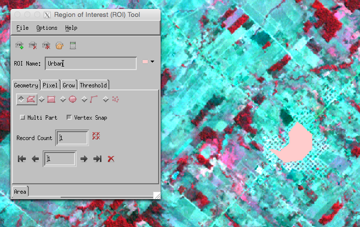
In envi, you need to define these classes via ROIs (Regions of Interest). Select the ROI tool:

and outline an ROI you want to define with the tool:

You may find the ‘N-D visualiser’ useful when doing this:

If you select only 2 bands to view, you will see informatyion similar to the scatterplot (i.e. 2-dimensional).

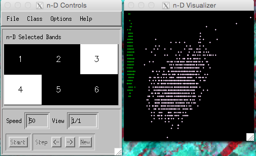
In such a view, you can readily ‘see’ how separable the classes might be.

In higher dimensions, the visualiser ‘rotates’ the view so you can get different perspectives on the classes

Note that you will want to create an ROI for each class you are interested in, but that yoy can ‘merge’ (or delete) classes once you have created them.

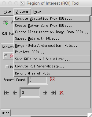
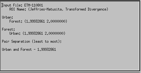
When you think you have a suitable set of ROIs, check the class separability:

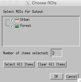
This outputs Divergence metrics between the classes you have defined. These values range between 0 and 2.0. As a guide to interpretation, values greater than 1.9 indicate good separability of classes. If class separability is less than this, you might consider splitting the classes for the classification and recombining them post-classification (e.g. have two classes: forest1 and forest2).

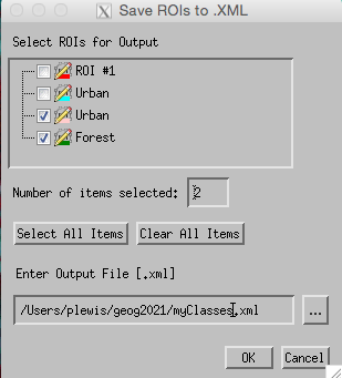
Then, make sure you save them (to xml format):

6.5. Image Classification

To perform a classification, first look at the options in the Toolbox:

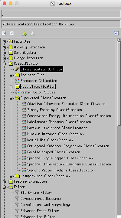
As a first attempt, try the Maximum Likelihood classifier.

A Tutorial is available that will take you through some of the other options.

For the Maximum Likelihood classifier, slect this itme from the Toolbox:

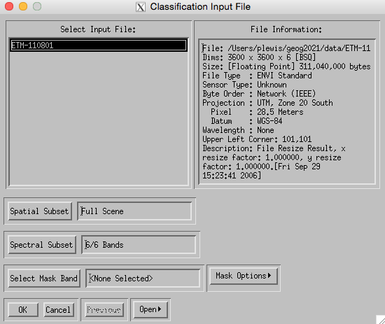
and perform any subsetting or masking that you might require.

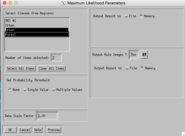
Then, select the Classes you want from the ROIs you have defined, along with making decisions about whether you want to save the result or not (if not, then just send it to ‘memory’, but it will not then be saved at the end of the session). If you do save the result, make sure you note down (in your notebook) what the file name was and what settings you used (e.g. which classes).

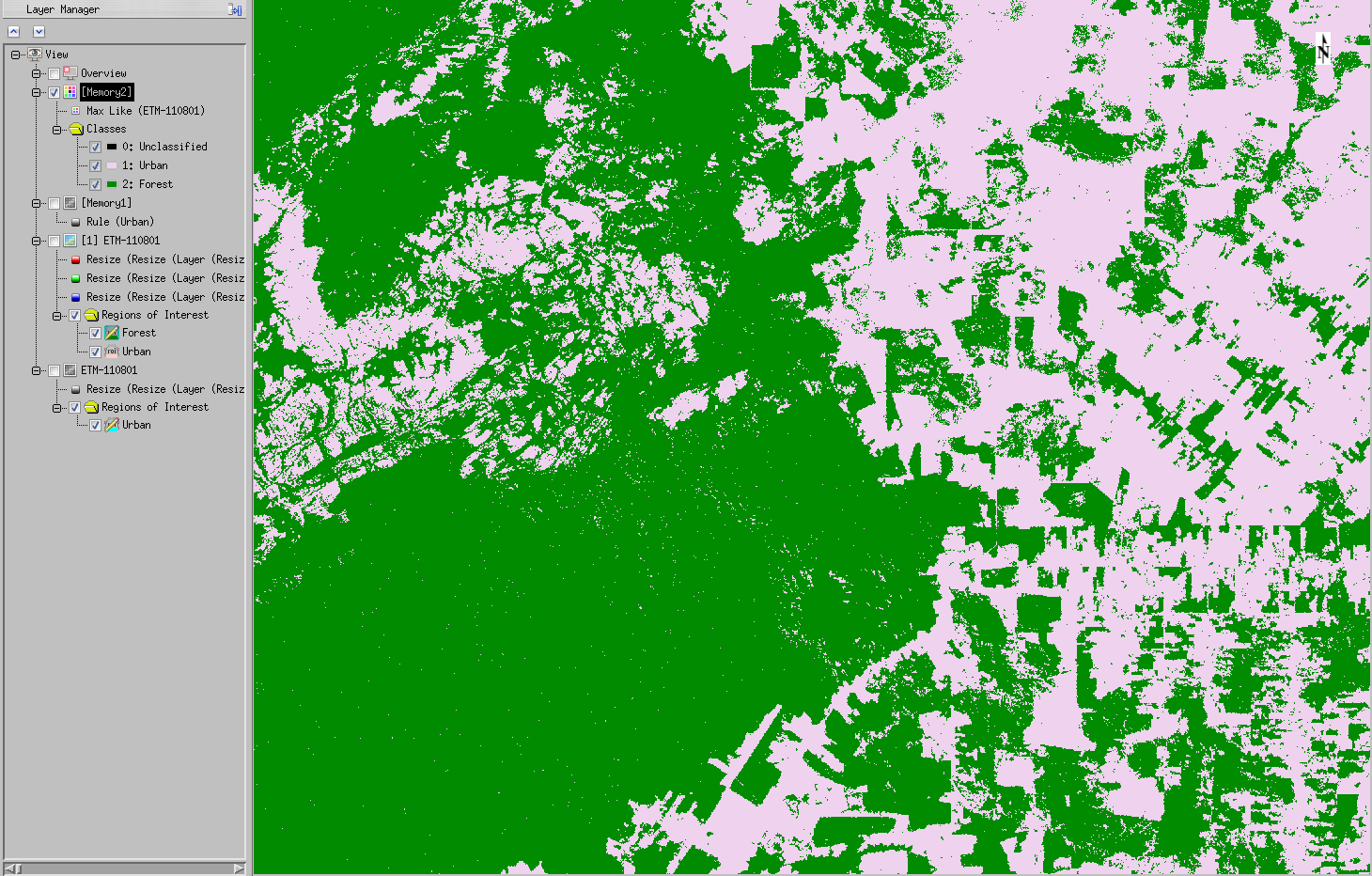
You should now have a classification result:

It is generally very instructive to visualise the ‘rule’ image associated with a result. This provides you with the reasoning the computer used to obtain the result it did.

For a method such as that used above, the training data are used to generate multivariate statistical distributions that we suppose to describe the full class. Each pixel then can be assigned a probability of class membership. The class which has the highest membership probability is usually assigned that class label.

What issues might occur if the probability of belonging to more than one class is very similar?

There appear to be topographic effects in the class probability images: why would that be so? and what might you do about it?

6.6. Accuracy Assessment

It is not very difficult to produce a classified map using earth observation data. You have now been through the process ofsupervised classification (using one method).

How can we tell how good this is though?

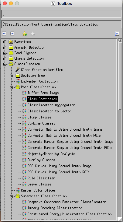
One thing you may wish to do is to examine the post-classification class statistics:

There are various other options that you may find useful to explore in the Post Classification section of the toolbox.

A vital part of the classification process though is an assessment of classification accuracy.

This is generally done as a confusion matrix.

In setting this up, you need either to have a ground truth ‘image’, or a set of ROIs that can be used for ground truth.

You should first generate a new (independent) set of ROIs (or better still, use random samples) for your classes. If you use random samples, you can check what you think the land cover class should be using Google Earth/Maps as above.

Once you have your confusion matrix, make sure that you understand what it is telling you (and as far as possible, why that is so).

If the classification result seems poor, you can go back and edit your settings or class definitions and re-try, but try to keep the ROIs you use for checking independent of this process.

Make sure you understand the terms we use to describe the different accuracies shown in the confusion matrix, and also what a kappa coefficient is.

6.7. Further Work

In this practical, you have gone through the process of performing an image classification and assessing its accuracy.

To finish the practical, you should classify both of the Landsat datasets you have, and calculate the change in forest area between the two dates. Since you have an accuracy assessment, it should be feasible for you to put an uncertainty on that estimate of change.

6.8. Summary

The main aim of this practical is to reinforce your understanding of the classification process and for you to gain practical experience at this.

It would be worthwhile exploring some of the options you have available (e.g. try some different classifiers).

Since there is quite a lot of ‘button clicking’ in this exercise, make sure that you understand what you are doing and why you are getting the result you do – there is very little value in the exercise otherwise!

If you have questions, ask the staff!

If you are very interested in change detection, you could explore the change detection options in ENVI.