![]()
5. Classification using ENVI 5.5
5.1. Aims
After completing this practical, you should be able to analyse one or more image datasets using classification methods. This includes learning to identify land cover classes in a dataset and consider class separability (using histograms, scatterplots and other tools), and applying and assessing a classification product using Envi.
5.2. Data
The datasets you need for this practical are available from the Classification data (Rondônia) folder on moodle or you can download them individually:
You should download these data and put them in a directory (folder) that you will remember!
The data you will be using are:
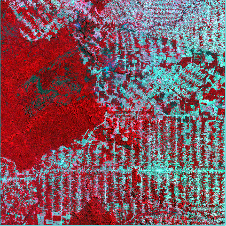
six wavebands of a Landsat TM image over Rondonia, Brazil, imaged on 25th July 1992. The data are at an original pixel spacing of 28.5 m.
six wavebands (nominally the same wavelengths) of a Landsat ETM image with the same spatial resolution, covering the same spatial extent. These data were obtained on 11th August 2001.
Digital Elevation model (DEM) data, obtained by RADAR interferometry from data on the SRTM (Shuttle Radar Topography Mission), are also available for the site. The data have been resampled to the same reolution and area as the TM/ETM data above.
The wavebands are:
1 |
2 |
3 |
4 |
5 |
6 |
|---|---|---|---|---|---|
blue |
green |
red |
nir |
swir 1 |
swir 2 |
450-520 nm |
520-600 nm |
630-690 nm |
760-900 nm |
1550-1750 nm |
2080-2350 nm |
The extent of the imagery is (Lat/Lon):
The full SRTM data can be loaded into google earth, if you have access to this.
Although you have the data ‘pre-packaged’ for this practical, you can download your own datasets using the USGS Glovis tool:
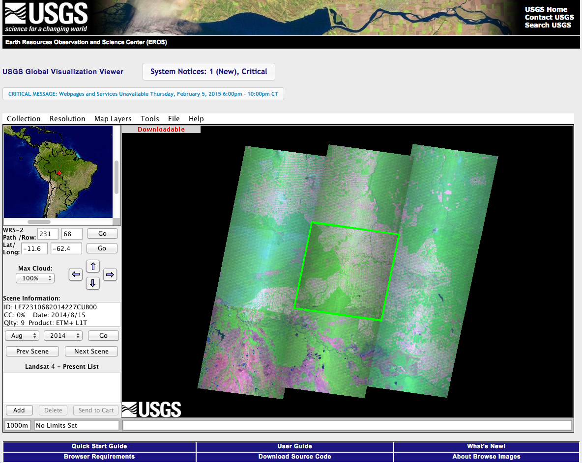
We can of course explore the area in Google Maps, which we may find useful for exploring the classification.
5.3. Introduction
*In this section, we load the image data we wish to explore*.
Importantly, we have the ability to map these changes from the archive of satellite data, particularly data from the Landsat series of satellites. An excellent introduction to visualising environmental change from Landsat data is given by Jeffrey Kluger.
Using data such as these, we can ‘track’ the changes in land cover over time.
For example, data produced by Google and Dr. Matthew Hansen at the University of Maryland which shows global maps of forest change (2000-2019) using Landsat data (see Science article), with red showing loss in 2019 through to yellow for the year 2000 (using pseudocolour), or with 2019 highlighted in aqua blue if you are viewing the default ‘Forest Loss Year (2019
Highlight) product. 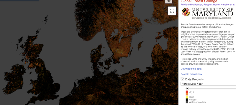
The purpose of this practical is for you to perform and test a land cover classification over this area, using data from two dates (1992 and 2001). The visualisations above show that there has been significant change since 2001 (and before 1992).
We will be doing this using separate classifications of the two image dates, but you should be thinking throughout about whether this is an appropriate method, and what else you might consider (especially if you had a long time series of data such as those shown in the animations).
We will be doing a supervised classification here.
The steps you will undertake are:
Examine the data and explore the spectral characteristics
Define a series of Regions of Interest (ROIs) describing the classes you wish to extract
Perform the classification
Test the result
First, obtain and then load the TM and ETM images of Rondonia noted above, along with the SRTM DEM file.
View the ETM image as a FCC.
You may need to edit the image file to associate the DEM data correctly. To do this, look under ‘Raster Management’ in the Toolbox, and edit the ENVI header (for the Landsat data). You should then edit the header attributes to associate the DEM with the image data.
[ ]: