3. Download data

In this section, you will learn how to order Landsat data from the USGS, including how to search only for the area we are interested in.

You will attempt to find two clear scenes (cloud-free or nearly so) for your area of interest.

You will then learn how to download the datasets.

Finally, we present one manual and one automated method for scaling the data, subsetting and producing a mask.

This is a skill you will need to complete the assessed coursework.

Once you have this skill, you can start collecting the datasets for the practical.

You do not need to use the ‘automated’ subsetting method: you can do everything manually if you wish.

3.1. Downloading and visualisation tools

The first task is to download the data that you will need.

There are several tools available to you for browsing and ordering Landsat data. See the USGS for a full description of the data products and where to order them.

You will most often be interested in surface reflectance products. These can be ordered through the USGS Earth Resources Observation and Science (EROS) Center Science Processing Architecture (ESPA) On Demand Interface.

The first time you visit the ordering service, you will need to register for an account. Make sure you remember the usename and password you used for registration!

Once at the USGS Earth Resources Observation and Science (EROS) Center Science Processing Architecture (ESPA) On Demand Interface site, make yourself aware of the information on surface reflectance.

3.2. Select Landsat Scenes

To select a particular landsat scene, go to the Earth Explorer site.

Enter the place you are interested in, in the Search Criteria (e.g. try: London, England) or select an area on the graphic using the Use Map polygon option.

Under Data Sets, look in Landsat -> Collection 1 Level 1 and check all of the boxes that have surface reflectance data. This will be for different sensors in the Landsat series (LS4-5, LS-7, LS-8).

You may wish to set a cloud cover limitation (e.g. 10%) under Additional Criteria.

Click on ‘Results’ and look at a few of the images. In particular, you should look at which ``PATH` and ROW <https://landsat.usgs.gov/landsat_acq>`__ is appropriate for the area you want data for. This could, for example be

Path 201
Row 24

Now, you can go back to the Search Criteria and enter just the path/row that you want, and/or just go through and add the files you want to download to the basket. This is the bar you have: Footprint, Overlay, Compare, Metadata, Download, Bulk Download, Order Scene, Remove

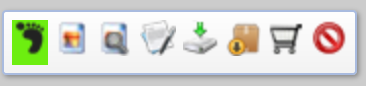
The first two are good for looking at, checking the cloud cover, and image cover. Choose either Download, or Bulk Download to get the full image. Select the GeoTIFF, the largest file.

For bulk download you can the view the basket, and submit the order. For this practical I suggest the DOWNLOAD option, getting immediate access to an image.

You should first try the Bulk Donwload with a small number of datasets, but it is quite straightforward to order many scenes if you need them.

If the order has worked, you will receive an email and also a notification when the data are ready for download. The order can be checked here https://dds.cr.usgs.gov/queue/orders/.

Once you get confirmation that the order is ready (this can, at times, take days but is usually less), you can then download the dataset.

3.3. Download ordered data

You can simply download the data by following the links in the email you receive.

Alternatively, there are various tools you can use for bulk download.

One example is `espa-bulk-downloader <>`__, which is a python script. You use this, e.g.:https://code.usgs.gov/espa/bulk-downloader

download_espa_order.py -e p.lewis@ucl.ac.uk -d ~/Downloads -u p.lewis@ucl.ac.uk -p MYPASSWORD -o ALL

This is very handy if you wish to download a large amount of data to a remote network.

You can also use the USGS download app https://dds.cr.usgs.gov/bulk/, though this is unavailable on UCL Desktop.

3.4. Unpacking Downloaded data

The images from USGS come intially in a compressed tar.gz file. This can be unpacked using either a command line or terminal on a unix or Mac machine. For UCL Desktop use the Command Prompt app.

We will navigate to the downloaded file using typed commands. There exists a typed command for everything you may wish to do. First to get to the correct file system N: then get to the data folder cd GEOG0027/data (or wherever you downloaded the data) List all the files in this directory dir The downloaded file will be in this list. Then extract all the images using tar -zxvf  DOWNLOADED_FILE.tar.gz (changing the tar.gz file name to the file you downloaded). You will see tiff files for each band.

3.5. Fixing Landsat 7 SLC issues

If you make use of Landsat 7 data (after slc failure in 2003 you may wish to perform a ‘gap filling’ on the dataset prior to use.

There are many such algorithms. One you can use quite easily is mentioned here.

To use this, download the file Landsat Gapfill IDL Model, either directly to, or copied to your envi/extensions directory (change folder permission if needed). From Desktop@UCL, your envi extension folder should be N:/.idl/envi/extensions5_5 or check your directory settings as shown below:

On a unix machine, this will involve e.g.:

cp ~/Downloads/landsat_gapfill.sav ~/.idl/envi/extensions5_5

Then, you should find the model available to you the next time you run envi, under the extensions menu. To view the toolbox you need to press F3. You may need to use the on-screen keyboard on UCL Desktop to do this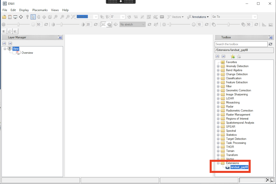

You may need to run this file seperately for each waveband.

Once the extension is run it will wish to save the corrected image. You can rewrite the original image, or created a fixed version. As you can see we are creating a lot of data, so you may wish to make more folders to keep it all organised and tidy.

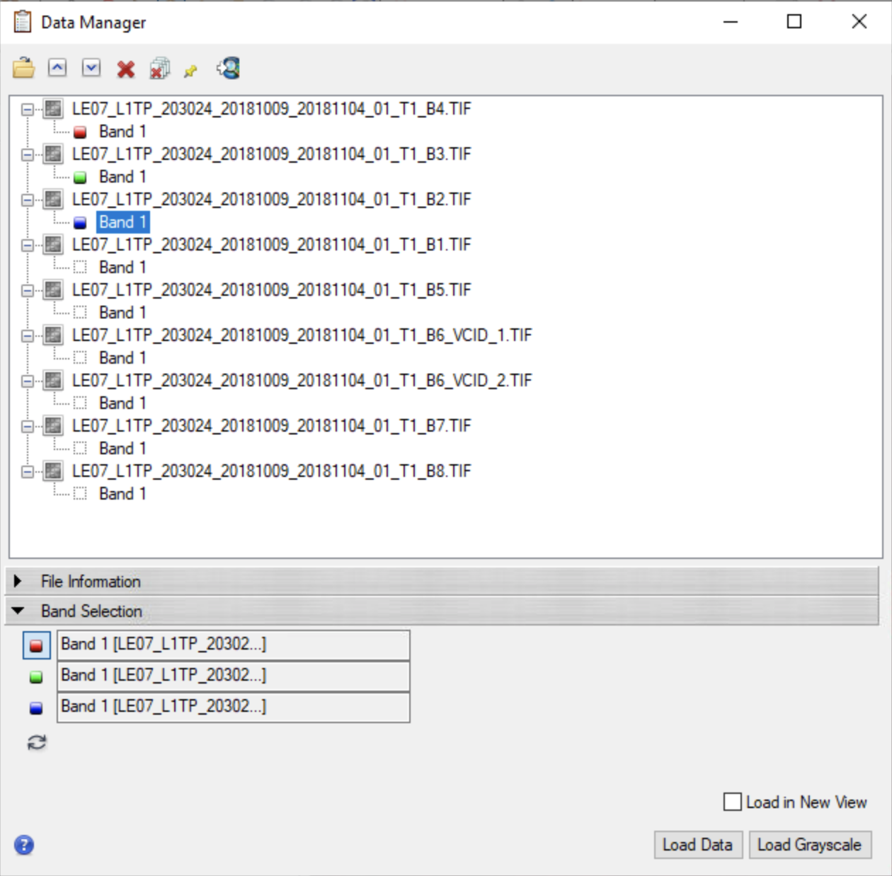
3.5.1. Viewing Multiband Files

To view a composite image from the seperate .tiff files we use the Data Manager

To work out which file represents which wavelength read the documentation here https://www.usgs.gov/faqs/what-are-band-designations-landsat-satellites

Can you recreate a true colour image, or one of the diagnostic images discussed in this weeks lecture? Remember the skills presented in last weeks practical.

3.6. Download Scenes

You will be sent an email from the USGS.

You must keep this email to show evidence that you have ordered the data.

The email will give you a web address that will look something like http://espa.cr.usgs.gov/ordering/order-status/p.lewis@ucl.ac.uk-01112017-113611-005.

If you have recent or active orders, this web page should show you the status for each file (wait until it says ‘complete’).

Then, you can download the file (using the Download link).

You must keep a record of the download links to show evidence that you have ordered the data, e.g.:

http://espa.cr.usgs.gov/orders/f.bloggs@nasa.gov-0101502242983/LE71220442000306-SC20150224104838.tar.gz

Save all of the download links in a file to include in your report.

The filename will be something like:

LE71220441999255-SC20150217105511.tar.gz

There is no need to ‘unzip’ or ‘untar’ the file: just download it for the moment.

Make sure you remember which directory you have downloaded the data to.

You should probably download the datasets to your N: Drive (or DATA disk in the Unix lab), or you might run out of quota, or at least move the files to the N: Drive (or DATA disk) soon after.

As the files are quite large, it may take some minutes to download each scene.